Simulating a Simple \(2\times 3 \times 2\) Quantum Neural Network

Here we give a short overview of a somewhat new architecture for quantum neural networks, in the form of a simple example.
Quantum neural networks (QNNs), as proposed in Kerstin Beer et al's, Training Deep Quantum Neural Networks, are a newly proposed framework for NISQ and future quantum computers capable of learning arbitrary completely positive linear maps on quantum state spaces (i.e. quantum operations).
Quantum Operations
In most introductory quantum courses, the relevant quantum states representing the system are taken as vectors (usually denoted as a bra such as \(\vert\psi\rangle\)) in some Hilbert space. These pure quantum states in closed systems then evolve according to arbitrary unitary maps \(U\), which act on the corresponding state space. Thus, we have the following map for state evolution over time: \[ \vert\psi\rangle\rightarrow U \vert\psi\rangle\] This map, however, isn't the most general model for all quantum systems of interest, since we're often interested in an effective subsystems of some larger quantum system.
For example, if we're only interested in a single qubit, it's relatively hard to completely close off the qubit from it's environment (especially if we intend to act on it and measure it ourself!). In fact, the single qubit's state will, in general, quickly become part of a larger quantum system (this larger part is often termed the environment), and evolve in concert with this larger system.
Thus, a more general map for the time evolution of some quantum system of interest should allow for those in which we only see a small subsystem of a larger quantum system that is evolving in some larger Hilbert space encapsulating not only it's own state space but also it's environment's. This more general map then takes the form below: \[ \rho_{sub}\rightarrow \text{Tr}_{env}\left[U\left(\rho_{sub}\otimes \rho_{env}\right)U^{\dagger}\right] \]
So the single qubit's state is really more appropriately modeled as a reduced density matrix, where the time evolution really occurs due to some unitary action on the larger quantum state of the qubit tensored with it's environment; and with the reduced density matrix being that returned after a partial trace over the environment's disjointed state space.
Quantum Neural Networks
Considering the general map above for time evolution, we'd like some framework for an algorithm that can effectively learn a certain map given a set of data generated from the map's associated operation. This makes clear what sort of data we intend to fit, the structure of which is made clear below. Of course, once we have an appropriate set of data, we also need some way to measure our algorithm's performance in matching the data, a point to be discussed immediatley after.
Data
The data we wish to learn from is that generated by some particular quantum operation. We thus need a set of input states (known before the operation) and output states (input states after the operation); and hence need a set of data of the form:
Cost
We now need a metric by which we may judge the performance of the network on the training data.
For data based on mixed states, we may replace the above with an averaged fidelity between output and target states. Explicitly then, for this case, we have the following: \[ C=\frac{1}{N}\sum_{i=1}^{N}\left(\text{Tr}\left[\sqrt{\sqrt{\rho_i}\rho^{out}_i\sqrt{\rho_i}}\right]\right)^2 \]
\(2\times 3\times 2 \) QNN Example
Below, the basics of the framework are covered in a simple example, closely following the presentation given by Ramona Wolf.
Our simple example of the model will consist of a two-qubit input state, one three-qubit hidden layer, and a two-qubit output state.

Since there are \(3_{(int)} + 2_{(out)} = 5\) qubits beyond the input layer, there are 5 constituent unitaries composing the QNN: with \(U^1_1\), \(U^1_2\), and \(U^1_3\) for the intermediate layer; and with \(U^{out}_1\) and \(U^{out}_2\) for the final layer. Unitaries for the intermediate layer \(U^1_m\) then act non-trivially on a state space of dimension \(2^{2+1}\times2^{2+1}\) but are tensored with identity in the rest, resulting in a matrix of dimension \(2^{2+3}\times2^{2+3}\). Similarly, unitaries for the output layer \(U^1_m\) then act on a state space of dimension \(2^{3+1}\times2^{3+1}\) but are tensored with identity in the rest, resulting in a matrix of dimension \(2^{3+2}\times2^{3+2}\).
These 5 unitaries then require us to construct 5 training matrices \(K_m^{\ell}\), each corresponding uniquely to one of the above unitaries.
Forward Pass
The action of the first step is to take the tensor product of the arbitrary input state \(\rho_{in}\) with a fiduciary (cleanly initialized), three qubit ground state \(\vert 000\rangle \langle 000 \vert \), and then apply three unitaries of dimension \(2^{2+1}\) which act on the input state and the first, second, and third intermediate state vectors, respectively (with identity in the rest) and in that order (because unitaries won't neccessarily commute and the convention is to apply from top to bottom for each layer). The partial trace is then taken over the input state's Hilbert space.
This resulting state represents the intermediate quantum state of the QNN. This is then tensor producted with the output state, which is also initialized as the ground state of a two-qubit Hilbert space. Two more \(2^{1+2}\) dimensional unitaries are then applied to the intermediate qubit's and the top and bottom qubits of the output state, respectively (in order from top to bottom), and the partial trace over the intermediate state space is then taken. The resulting \(2^{2}\) dimensional state \(\rho_{out}\) is then the output of this simple model.
This forward pass thus takes the following form:
Training Matrices
We now would like to update the constituent unitaries by some map which allows us to improve the cost on the training data. We define this map as \[U_{m}^{\ell} \rightarrow e^{-\epsilon K_{m}^{\ell}}U_{m}^{\ell}\] where each unitary thus has a corresponding training matrix.
For the intermediate layer's unitaries, we have the corresponding training matrices:
And then for the output layer's unitaries, we have the corresponding training matrices:
Adjoint Layer
Since there is only one intermediate layer for the given structure, there is only one relevant adjoint map, analogous to a backward pass from the output layer to the intermediate layer. We now define this adjoint map as follows:
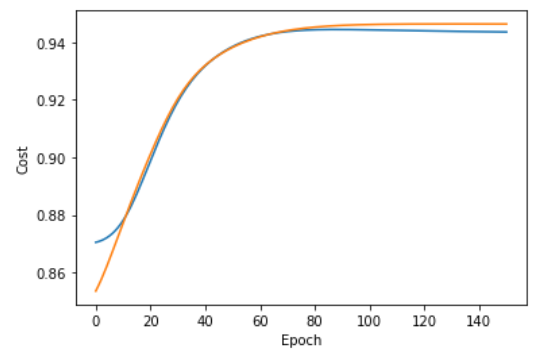
Simulated Results
For a random set of initial unitaries applied to a set of data generated via
Further Resources
For a stand-alone document that covers the same material here in more depth, see this introductory article. The original paper can be found here.
